Hi folks,

This is the weekly digest for my blog, Irrational Exuberance. Reach out with thoughts on Twitter at @lethain, or reply to this email.

Posts from this week:

- Modeling impact of LLMs on Developer Experience.

Modeling impact of LLMs on Developer Experience.

In How should you adopt Large Language Models? (LLMs), we considered how LLMs might impact a company’s developer experience. To support that exploration, I’ve developed a system model of the developing software at the company.

In this chapter, we’ll work through:

1. Summary results from this model
2. How the model was developed, both sketching and building the model in a spreadsheet. (As discussed in the overview of systems modeling, I generally would recommend against using spreadsheets to develop most models, but it’s educational to attempt doing so once or twice.)
3. Exercise the model to see what it has to teach us

Let’s get into it.

This is an exploratory, draft chapter for a book on engineering strategy that I’m brainstorming in #eng-strategy-book. As such, some of the links go to other draft chapters, both published drafts and very early, unpublished drafts.

Learnings

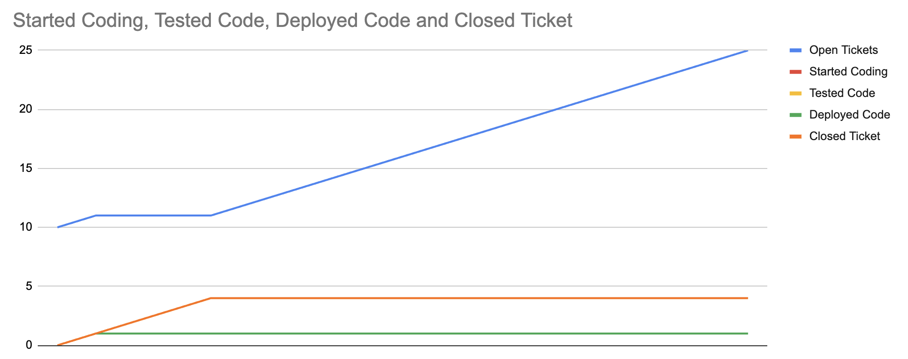
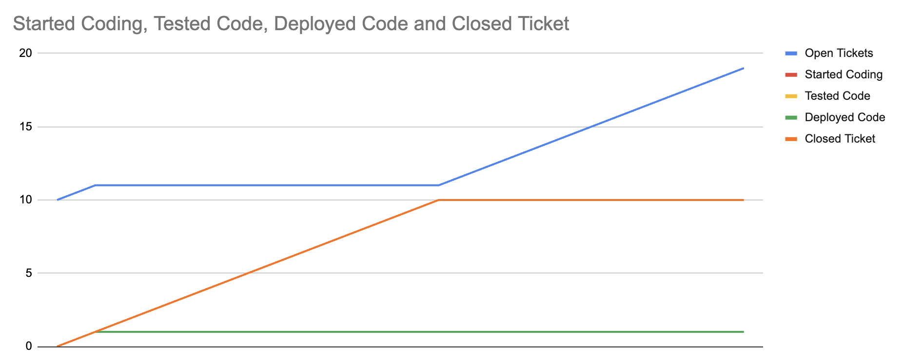
This model’s insights can be summarized in three charts. First, the baseline chart, which shows an eventual equilibrium between errors discovered in production and tickets that we’ve closed by shipping to production. This equilibrium is visible because tickets continue to get opened, but the total number of closed tickets stop increasing.

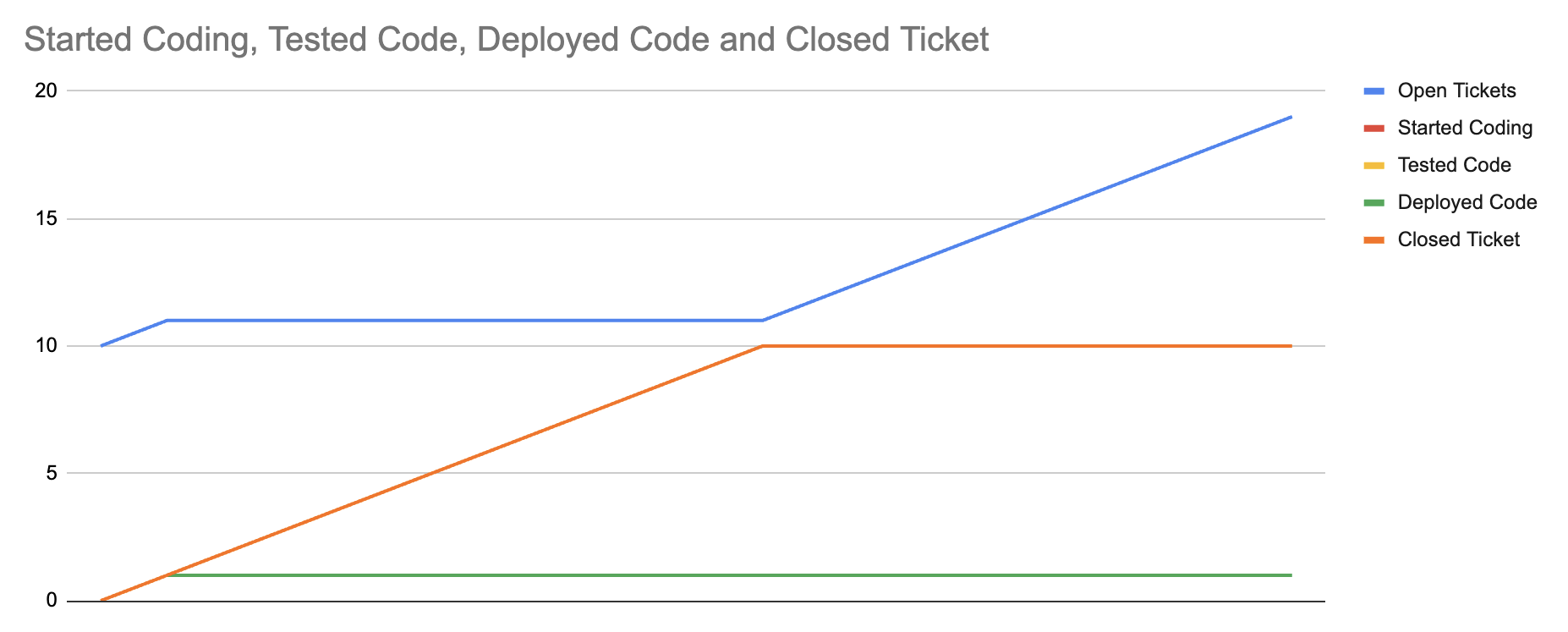
Second, we show that we can shift that equilibrium by reducing the error rate in production. Specifically, the first chart models 25% of closed tickets in production experiencing an error, whereas the second chart models only a 10% error rate. The equilibrium returns, but at a higher value of shipped tickets.

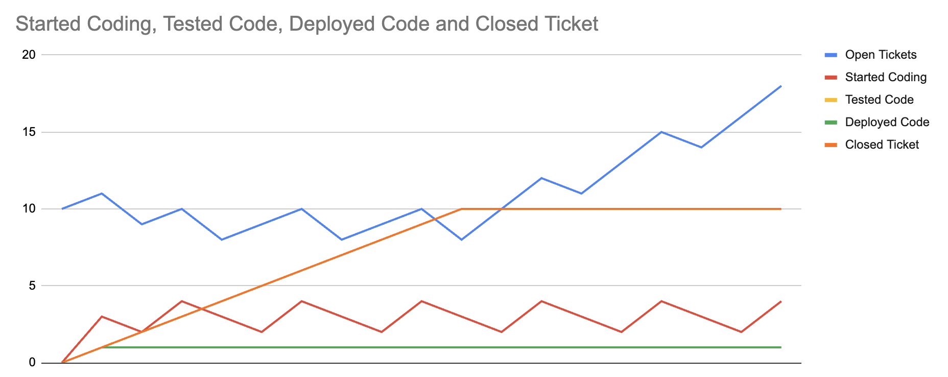
Finally, we can see that even tripling the rate that we start and test tickets doesn’t meaningfully change the total number of completed tickets, as modeled in this third chart.

The constraint on this system is errors discovered in production, and any technique that changes something else doesn’t make much of an impact. Of course, this is just a model, not reality. There are many nuances that models miss, but this helps us focus on what probably matters the most, and in particular highlights that any approach that increases development velocity while also increasing production error rate is likely net-negative.

With that summary out of the way, now we can get into developing the model itself.

Sketch

Modeling in a spreadsheet is labor intensive, so we want to iterate as much as possible in the sketching phase, before we move to the spreadsheet. In this case, we’re working with Excalidraw.

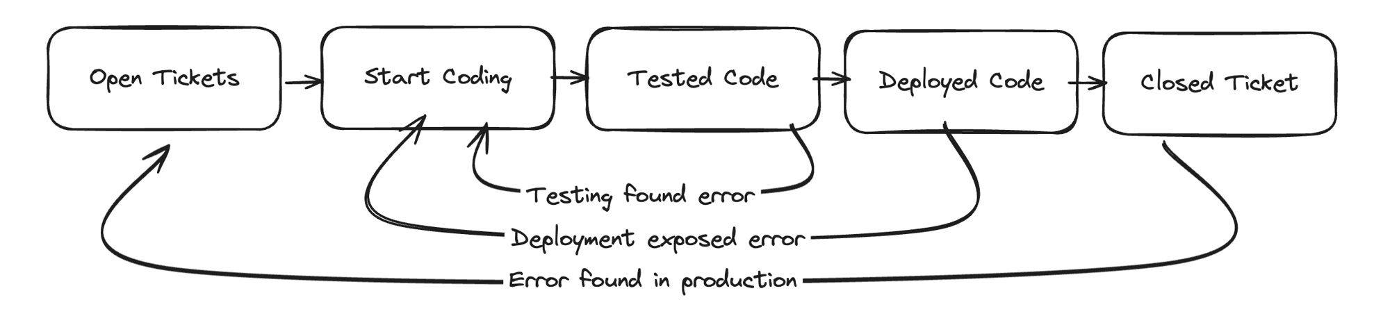
I sketched five stocks to represent a developer’s workflow:

1. Open Tickets is tickets opened for an engineer to work on
2. Start Coding is tickets that an engineer is working on
3. Tested Code is tickets that have been tested
4. Deployed Code is tickets than have been deployed
5. Closed Ticket is tickets that are closed after reaching production

There are four flows representing tickets progressing through this development process from left to right. Additionally, there are three exception flows that move from right to left:

1. Testing found error represents a ticket where testing finds an error, moving the ticket backwards to Start Coding
2. Deployment exposed error represents a ticket encountering an error during deployment, where it’s moved backwards to Start Coding
3. Error found in production represents a ticket encountering a production error, which causes it to move all the way back to the beginning as a new ticket

One of your first concerns seeing this model might be that it’s embarassingly simple. To be honest, that was my reaction when I first looked at it, too. However, it’s important to recognize that feeling and then dig into whether it matters.

This model is quite simple, but in the next section we’ll find that it reveals several counter-intuitive insights into the problem that will help us avoid erroneously viewing the tooling as a failure if time spend testing increases. The value of a model is in refining our thinking, and simple models are usually more effective as refining thinking across a group than complex models, simply because complex models are fairly difficult to align a group around.

Reason

As we start to look at this sketch, the first question to ask is how might LLM-based tooling show an improvement? The most obvious options are:

1. Increasing the rate that tasks flow from Starting coding to Tested code. Presumably these tools might reduce the amount of time spent on implementation.

2. Increasing the rate that Tested code follows Testing found errors to return to Starting code because more comprehensive tests are more likely to detect errors. This is probably the first interesting learning from this model: if the adopted tool works well, it’s likely that we’ll spend more time in the testing loop, with a long-term payoff of spending less time solving problems in production where it’s more expensive. This means that slower testing might be a successful outcome rather than a failure as it might first appear.

   A skeptic of these tools might argue the opposite, that LLM-based tooling will cause more issues to be identified “late” after deployment rather than early in the testing phase. In either case, we now have a clear goal to measure to evaluate the effectiveness of the tool: reducing the Error found in production flow. We also know not to focus on the Testing found error flow, which should probably increase.

3. Finally, we can also zoom out and measure the overall time from Start Coding to Closed Ticket for tasks that don’t experience the Error found in production flow for at least the first 90 days after being completed.

These observations capture what I find remarkable about systems modeling: even a very simple model can expose counter-intuitive insights. In particular, the sort of insights that build conviction to push back on places where intuition might lead you astray.

Model

For this model, we’ll be modeling it directly in a spreadsheet, specifically Google Sheets. The completed spreadsheet model is available here. As discussed in Systems modeling to refine strategy, spreadsheet modeling is brittle, slow and hard to iterate on. I generally recommend that folks attempt to model something in a spreadsheet to get an intuitive sense of the math happening in their models, but I would almost always choose any tool other than a spreadsheet for a complex model.

This example is fairly tedious to follow, and you’re entirely excused if you decide to pull open the sheet itself, look around a bit, and then skip the remainder of this section. If you are hanging around, it’s time to get started.

The spreadsheet we’re creating has three important worksheets:

• Model represents the model itself
• Charts holds charts of the model
• Config holds configuration values seperately from the model to ease exercising the model after we’ve built it

Going to the model worksheet, we want to start out by initializing each of the columns to the starting value.

While we’ll use formulae for subsequent rows, the first row should contain literal values. I often start with a positive value in the first column and zeros in the other columns, but that isn’t required. You can start with whatever starting values are more useful for studying the model that you’re building.

With the initial values set, we’re now going to implement the model in two passes. First, we’ll model the left-to-right flows, which represent the standard development process. Second, we’ll model the right-to-left flows, which represent exceptions in the process.

Modeling left-to-right

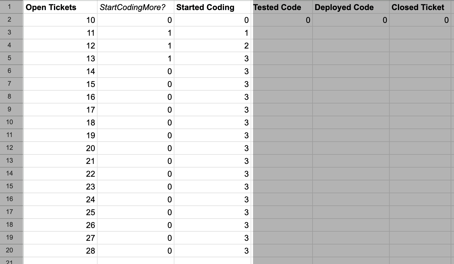
We’ll start by modeling the interaction between the first two nodes: Open Tickets and Started Coding. We want to have open tickets increased over time at a fixed rate, so let’s add a value in the config worksheet for TicketOpenRate, starting with 1.

Moving to the second stock, we want to start work on open tickets as long as we have at most MaxConcurrentCodingNum open tickets. If we have more than MaxConcurrentCodingNum tickets that we’re working on, then we don’t start working on any new tickets. To do this, we actually need to create an intermediate value (represented using an italics column name) to determine how many should be created by checking if the current in started tickets is at maximum (another value in the config sheet) or if we should increment that by one.

That looks like:

// Config!$B$3 is max started tickets
// Config!$B$2 is rate to increment started tickets
// $ before a row or column, e.g. $B$3 means that the row or column
// always stays the same -- not incrementing -- even when filled
// to other cells
= IF(C2 >= Config!$B$3, 0, Config!$B$2)

This also means that our first column, for Open Tickets is decremented by the number of tickets that we’re started coding:

// This is the definition of `Open Tickets`
=A2 + Config!$B$1 - B2

Leaving us with these values.

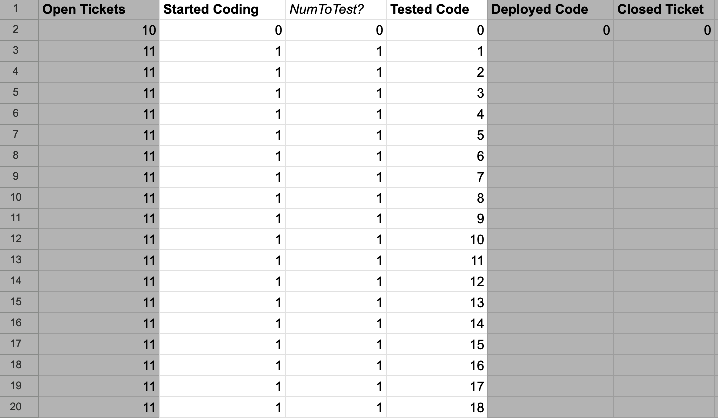
Now we want to determine the number of tickets being tested at each step in the model. To do this, we create a calculation column, NumToTest? which is defined as:

// Config$B$4 is the rate we can start testing tickets
// Note that we can only start testing tickets if there are tickets
// in `Started Coding` that we're able to start testing
=MIN(Config!$B$4, C3)

We then add that value to the previous number of tickets being tested.

// E2 is prior size of the Tested Code stock
// D3 is the value of `NumToTest?`
// F2 is the number of tested tickets to deploy
=E2 + D3 - F2

Moving on to deploying code, let’s keep things simple and start out by assuming that every tested change is going to get deployed. That means the calculation for NumToDeploy? is quite simple:

// E3 is the number of tested changes
=E3

Then the value for the Deployed Code stock is simple as well:

// G2 is the prior size of Deployed Code
// F3 is NumToDeploy?
// H2 is the number of deployed changes in prior round
=G2+F3-H2

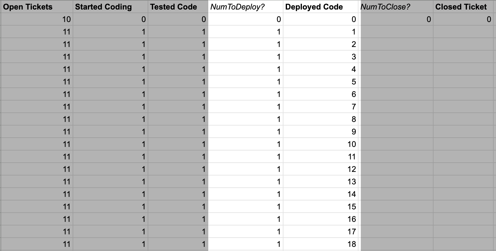
Now we’re on to the final stock. We add the NumToClose? calculation, which assumes that all deployed changes are now closed.

// G3 is the number of deployed changes
=G3

This makes the calculation for the Closed Tickets stock:

// I2 is the prior value of Closed Tickets
// H3 is the NumToClose?
=I2 + H3

With that, we’ve now modeled the entire left-to-right flows.

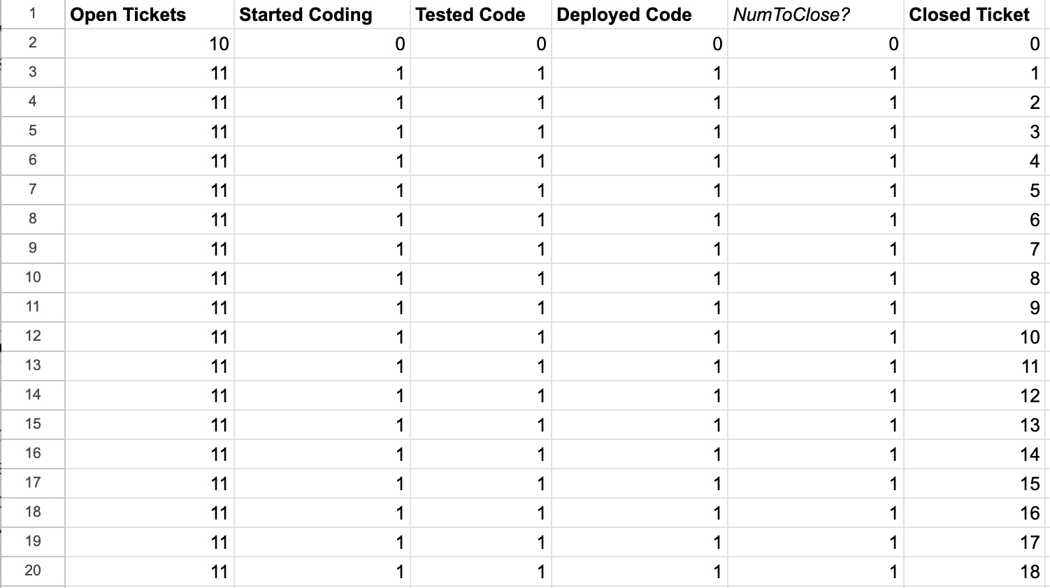
The left-to-right flows are simple, with a few constrained flows and a very scalable flows, but overall we see things progressing through the pipeline evenly. All that is about to change!

Modeling right-to-left

We’ve now finished modeling the happy path from left to right. Next we need to model all the exception paths where things flow right to left. For example, an issue found in production would cause a flow from Closed Ticket back to Open Ticket. This tends to be where models get interesting.

There are three right-to-left flows that we need to model:

1. Closed Ticket to Open Ticket represents a bug discovered in production.
2. Deployed Code to Start Coding represents a bug discovered during deployment. 3 Tested Code to Start Coding represents a bug discovered in testing.

To start, we’re going to add configurations defining the rates of those flows. These are going to be percentage flows, with a certain percentage of the target stock triggering the error condition rather than proceeding. For example, perhaps 25% of the Closed Tickets are discovered to have a bug each round.

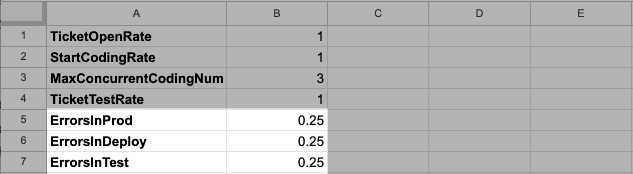
These are fine starter values, and we’ll experiment with how adjusting them changes the model in the Exercise section below.

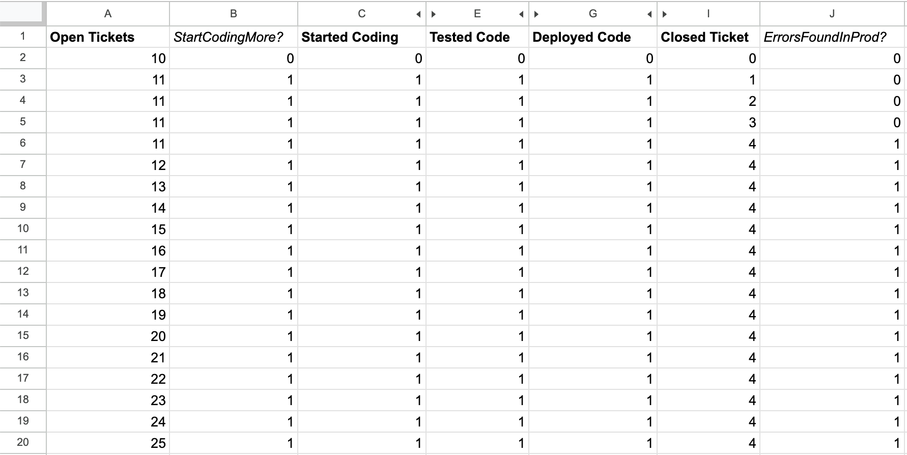
Now we’ll start by modeling errors discovered in production, by adding a column to model the flow from Closed Tickets to Open Tickets, the ErrorsFoundInProd? column.

// I3 is the number of Closed Tickets
// Config!$B$5 is the rate of errors
=FLOOR(I3 * Config!$B$5)

Note the usage of FLOOR to avoid moving partial tickets. Feel free to skip that entirely if you’re comfortable with the concept of fractional tickets, fractional deploys, and so on. This is an aesthetic consideration, and generally only impacts your model if you choose overly small starting values.

This means that our calculation for Closed Ticket needs to be updated as well to reduce by the prior row’s result for ErrorsFoundInProd?:

// I2 is the prior value of ClosedTicket
// H3 is the current value of NumToClose?
// J2 is the prior value of ErrorsFoundInProd?
=I2 + H3 - J2

We’re not quite done, because we also need to add the prior row’s value of ErrorsInProd? into Open Tickets, which represents the errors’ flow from closed to open tickets. Based on this change, the calculation for Open Tickets becomes:

// A2 is the prior value of Open Tickets
// Config!$B$1 is the base rate of ticket opening
// B2 is prior row's StartCodingMore?
// J2 is prior row's ErrorsFoundInProd?
=A2 + Config!$B$1 - B2 + J2

Now we have the full errors in production flow represented in our model.

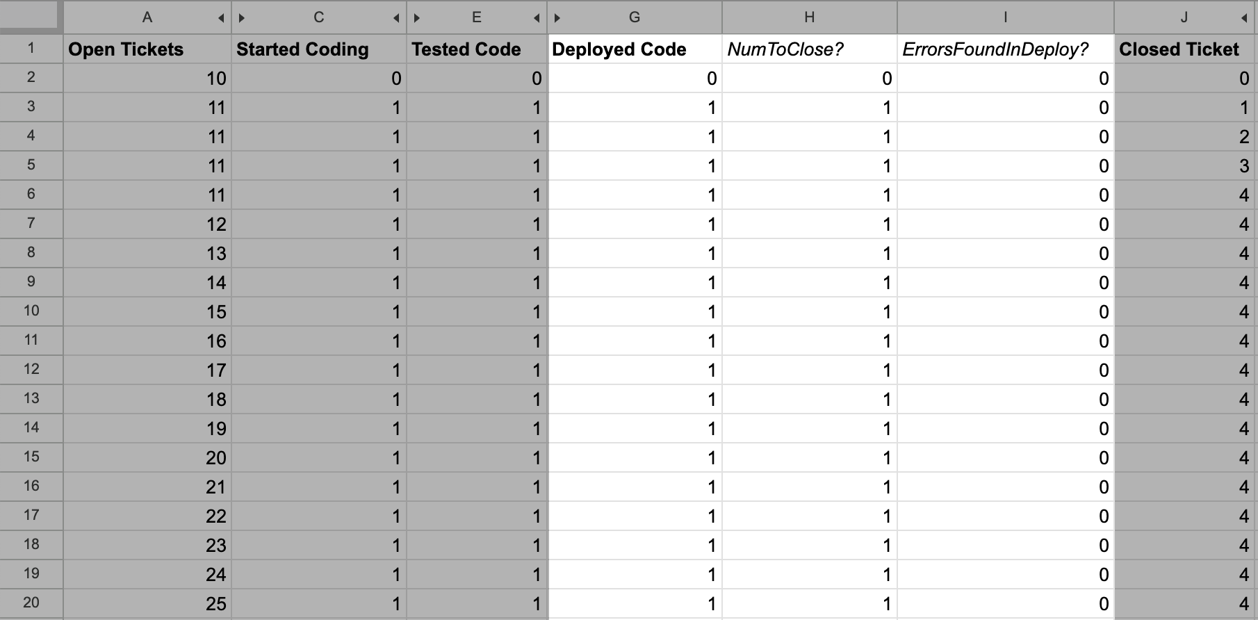
Next, it’s time to add the Deployed Code to Start Coding flow. Start by adding the ErrorsFoundInProd? calculation:

// G3 is deployed code
// Config!$B$6 is deployed error rate
=FLOOR(G3 * Config!$B$6)

Then we need to update the calculation for Deployed Code to decrease by the calculated value in ErrorsFoundInProd?:

// G2 is the prior value of Deployed Code
// F3 is NumToDeploy?
// H2 is prior row's NumToClose?
// I2 is ErrorsFoundInDeploy?
=G2 + F3 - H2 - I2

Finally, we need to increase the size of Started Coding by the same value, representing the flow of errors discovered in deployment:

// C2 is the prior value of Started Coding
// B3 is StartCodingMore?
// D2 is prior value of NumToTest?
// I2 is prior value of ErrorsFoundInDeploy?
=C2 + B3 - D2 + I2

We now have the working flow representing errors in production.

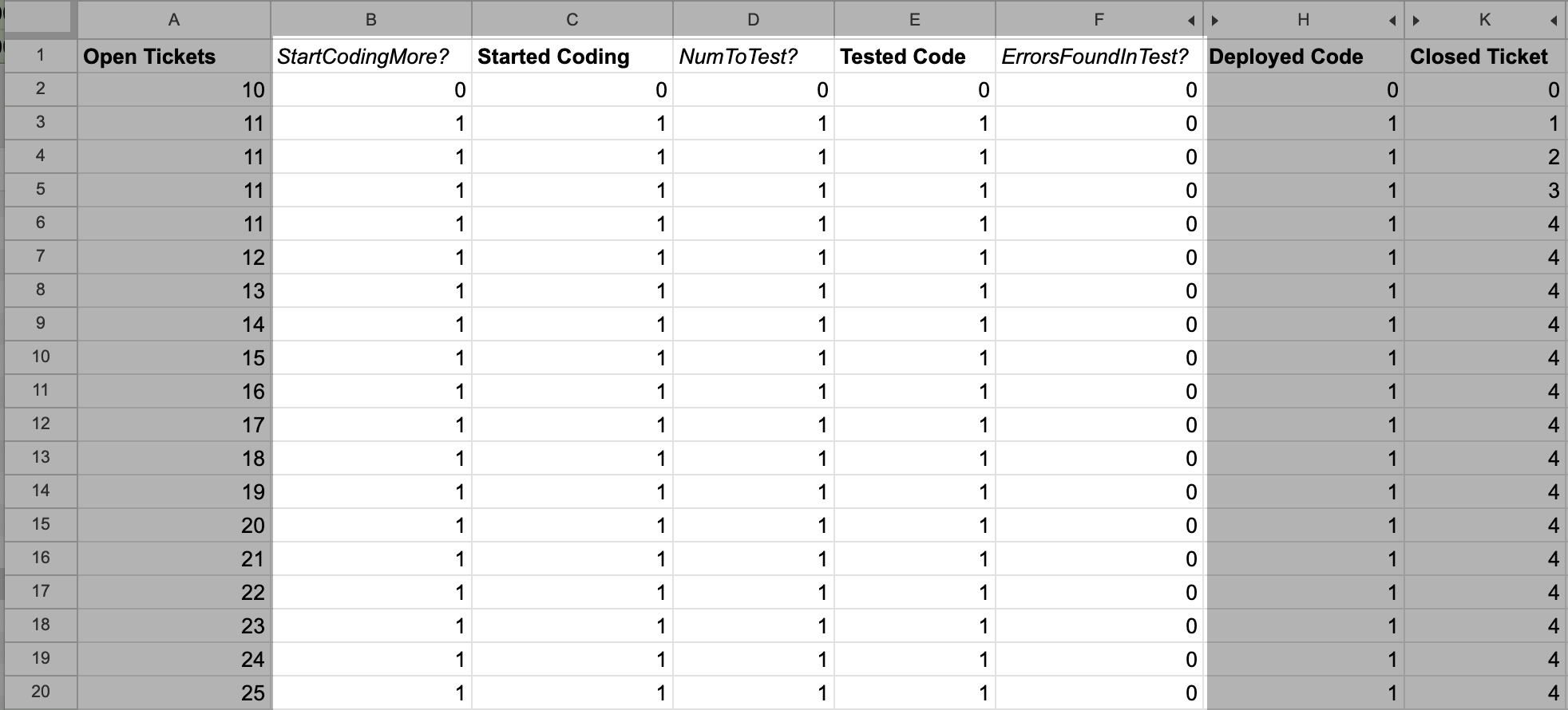
Finally, we can added the Tested Code to Started Coding flow. This is pretty much the same as the prior flow we added, starting with adding a ErrorsFoundInTest? calculation:

// E3 is tested code
// Config!$B$7 is the testing error rate
=FLOOR(E3 * Config!$B$7)

Then we update Tested Code to reduce by this value:

// E2 is prior value of Tested Code
// D3 is NumToTest?
// G2 is prior value of NumToDeploy?
// F2 is prior value of ErrorsFoundInTest?
=E2 + D3 - G2 - F2

And update Started Coding to increase by this value:

// C2 is prior value of Started Coding
// B3 is StartCodingMore?
// D2 is prior value of NumToTest?
// J2 is prior value of ErrorsFoundInDeploy?
// F2 is prior value of ErrorsFoundInTest?
= C2 + B3 - D2 + J2 + F2

Now this last flow is instrumented.

With that, we now have a complete model that we can start exercising! This exercise demonstrated both that it’s quite possible to represent a meaningful model in a spreadsheet, but also the challenges of doing so.

While developing this model, a number of errors became evident. Some of them I was able to fix relatively easily, and even more I left unfixed because fixing them makes the model even harder to reason about. This is a good example of why I encourage developing one or two models in a spreadsheet, but I ultimately don’t believe it’s the right mechanism to work in for most people: even very smart people make errors in their spreadsheets, and catching those errors is exceptionally challenging.

Exercise

Now that we’re done building this model, we can final start the fun part: exercising it. We’ll start by creating a simple bar chart showing the size of each stock at each step. We are going to expressly not show the intermediate calculation columns such as NumToTest?, because those are implementation details rather than particularly interesting.

Before we start tweaking the values , let’s look at the baseline chart.

The most interesting thing to notice is that our current model doesn’t actually increase the number of closed tickets over time. We actually just get further and further behind over time, which isn’t too exciting.

So let’s start modeling the first way that LLMs might help, reducing the error rate in production. Let’s shift ErrorsInProd from 0.25 down to 0.1, and see how that impacts the chart.

We can see that this allows us to make more progress on closing tickets, although at some point equilibrium is established between closed tickets and the error rate in production, preventing further progress. This does validate that reducing error rate in production matters. It also suggests that as long as error rate is a function of everything we’ve previously shipped, we are eventually in trouble.

Next let’s experiment with the idea that LLMs allow us to test more quickly, tripling TicketTestRate from 1 to 3. It turns out, increasing testing rate doesn’t change anything at all, because the current constraint is in starting tickets.

So, let’s test that. Maybe LLMs make us faster in starting tickets because overall speed of development goes down. Let’s model that by increasing StartCodingRate from 1 to 3 as well.

This is a fascinating result, because tripling development and testing velocity has changed how much work we start, but ultimately the real constraint in our system is the error discovery rate in production.

By exercising this model, we find an interesting result. To the extent that our error rate is a function of the volume of things we’ve shipped in production, shipping faster doesn’t increase our velocity at all. The only meaningful way to increase productivity in this model is to reduce the error rate in production.

Models are imperfect representations of reality, but this one gives us a clear sense of what matters the most: if we want to increase our velocity, we have to reduce the rate that we discover errors in production. That might be reducing the error rate as implied in this model, or it might be ideas that exist outside of this model. For example, the model doesn’t represent this well, but perhaps we’d be better off iterating more on fewer things to avoid this scenario. If we make multiple changes to one area, it still just represents one implemented feature, not many implement features, and the overall error rate wouldn’t increase.

That's all for now! Hope to hear your thoughts on Twitter at @lethain!